[Position paper] Dynamic life cycle assessment explained
Current practice in the building sector analyses impact over an assessment period without taking into account how these impacts change over time. Consuming 3000 kWh per year generates the same impacts in Y+1 as in Year 0, regardless of whether this energy is consumed in winter or in summer, during the week or at the weekend, during the day or night. This is a static LCA method. Dynamic LCA takes time variations into account on several levels.
1. Processes taking place in the system under study
The processes related to energy and water consumption vary greatly, depending on building use (housing, offices, etc.). Simplifying the calculation of the environmental balance sheet by considering annual water consumption does not result in any major errors as the technologies used to produce drinking water and treat waste water change little over time (and water consumption is much the same whether or not it rains). The same cannot be said for electricity, the production mix of which varies considerably (cf. data from RTE, France’s transmission system operator). A dynamic model, for example with hourly time steps, significantly improves the precision of the calculation: the difference between static and dynamic LCA may reach 40% (Roux et al., 2016a).
Beyond these variations over a day, week or year, there are also long-term variations (over several decades) related to the energy transition (Roux et al., 2016b). There are therefore plans to adjust the electricity generation mix by increasing the share of renewable energy sources. This is also the case for gas. Climate change also brings about a change in air-conditioning and indeed heating requirements.
Simplifying assumptions may be considered to prevent the calculation process from becoming overburdened. For example, knowing whether a product was produced six months or one year before the building work does not appear to have a significant impact on the LCA results.
Waste processing after a building’s long life span will most likely be different to what occurs today, which may give rise to a comparison of scenarios, as part of a sensitivity analysis, or an uncertainty estimate. Generally speaking, the processes taking place in the distant future are more uncertain. As regards these future processes, as a precaution, potential improvements resulting in impact reductions may not be factored in as they are only assumed and remain uncertain. This in turn leads to considering an overestimate of impacts (e.g. the impacts of current processes), supposing that the environmental performance of the processes will be improved in the future.
2. The life cycle inventory
The variation in processes leads to a variation in the life cycle inventory (cf. RTE data on CO2 emissions per kwh generated in France ).
Assessing an inventory hour by hour would make the calculation too unwieldy, and is only justified if characterization factors (used to convert emissions to impacts) vary greatly over time. This may be the case for volatile organic compound emissions, which break down according to the level of sunlight to form ozone which is harmful to health. In general, emissions do not vary according to sun exposure, therefore it is deemed sufficient to use an annual average in most cases. Wood heating causes more emissions in winter, when there is a lower level of sunlight, which may give rise to a more precise analysis if there is data on the variation of characterization factors according to sunlight.
3. Impact indicators
Certain physical or chemical phenomena such as the breakdown of some substances in the air, water or earth may vary over time according to weather conditions. As mentioned above, this is the case for the formation of photochemical ozone. Impacts may be calculated on an hourly basis according to sunlight (over a typical climatic year, for instance). This requires a modelling of characterization factors, and therefore supplementary research.
As regards global warming, the use of indicators as recommended by the IPCC does not take into account a potential variation of the impact according to the date of the emission. Certain exploratory methods consider a discount rate as in economic studies (one kilogram of CO2 emitted today is worth more than one kilogram emitted in fifty years) or no longer count impacts beyond a set cut-off point (e.g. in 100 years). This type of approach is highly questionable and there is no consensus of opinion within the scientific community. These methods give less importance to impacts affecting future generations, which runs counter to the principle of sustainable development. If impacts are not considered beyond a timeframe of 100 years[1] , does this equate to leaving future generations an “environmental debt”? This is a political choice, that cannot be justified by science.
[1] The indicators developed by the IPCC operate with a rolling time horizon, for example 100 years for Global Warming Potential, GWP100. The effects of an emission are integrated over the 100 following years, regardless of the date of this emission, and not solely over a set time horizon of 100 years from a building’s construction date. By considering this set time horizon, the effect of an emission taking place 50 years after construction is only integrated over the following 50 years, instead of 100 years, which underestimates the impact on future generations.
Examples comparing regulatory dynamic LCA and physical dynamic LCA
- 5-cm increase in glass wool for block walls (internal insulation and plasterboard)
Over one square metre, a 5-cm increase in thickness represents roughly 600g of glass wool, the production, transportation and implementation of which generates around 0.82 kg of CO2 in year 0 of the life cycle.
Increasing thickness from 15 cm to 20 cm brings about a reduction in annual heating requirements of around 2 kWh per m² of wall for a typical individual house in the Paris region. If heating is generated by a heat pump (the most common system under the 2012 thermal regulations for buildings and most probably under the 2020 environmental regulations), the corresponding reduction in electricity consumption is around 0.8 kWh (per year). The reduction in greenhouse gas emissions is 200g of CO2per kWh of electricity saved with the physical dynamic model (for heating, with an increased use of more carbonated resources in peak periods) and 79g CO2/kWh with the regulatory calculation in the first year. This amount decreases over the years according to the regulatory “dynamic” indicator, but remains constant in the physical LCA (the impact on global warming does not depend on the emission date).
The result is presented in the graph below:
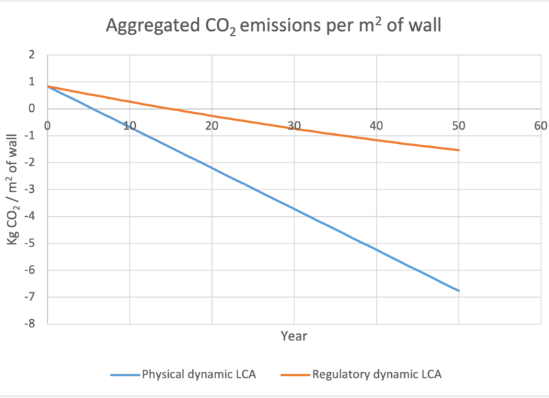
The initial CO2 emission is gradually offset by the energy saved through thermal insulation. However, according to the regulatory calculation, it takes 15 years to achieve this offsetting, whereas the carbon payback time is only 5 years with the more physical calculation. Ultimately, over the 50 years, the insulator will cut emissions 7 times more than the quantity emitted for its production according to the physical calculation, compared to only 1.5 times more with the regulatory calculation.
- Comparison between double and triple glazing
The production of one square metre of glazing generates around 11kg of additional CO2 for triple glazing compared to double glazing, but triple glazing (in this example installed on the north-facing façade of a typical individual house in the Paris region) cuts heating requirements by roughly 15 kWh and consumption by approximately 6 kWh (if a heat pump is used). The assessment of triple glazing compared to double glazing is therefore as follows for the two methods (the impacts related to a replacement of the window after thirty years are taken into account):
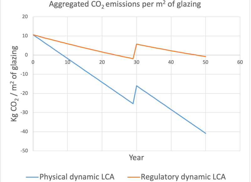
If a life span of 30 years is considered for the glazing[2], there is no added benefit of triple glazing according to the regulatory calculation as it results in higher overall emissions over the building’s entire life cycle. Conversely, the physical calculation demonstrates that triple glazing “pays for itself” in less than ten years, and that the reduction of emissions over the life cycle is roughly four times the amount initially emitted.
In both cases (insulation thickness and selection of glazing), the regulatory calculation shifts the environmental optimum towards a lower energy performance compared to the physical calculation. Physical dynamic LCA considers the increase in electricity consumption impacts in the colder months (more carbonated generation in peak periods), while the regulatory “dynamic” LCA decreases them over the years (global warming is no longer considered beyond 100 years). Due to this decrease in impacts, the regulatory calculation gives less value to energy-saving technologies or local renewable energy generation.
[2] Value considered in the regulatory database and in the physical LCA.
In short
As a dynamic thermal simulation may be used in addition to the regulatory approach, LCAs may be conducted on a more physical basis with a view to assisting project design. The physical dynamic LCA rolled out in the Pleiades ACV EQUER tool considers time variations for energy consumption, electricity generation processes and related environmental impacts (seasonal, weekly and hourly variations, long-term prospective scenarios).
Bibliography

CES

CES